UC-2.5 — Descriptive Statistics of Samples Across Databases
Module: 2 – Exploratory Analysis: Ranking the Functional Potential of Samples and Compounds
Visualization type: Interactive box-and-scatter (jitter) plot of unique KO counts
Primary inputs: BioRemPP, HADEG, and KEGG results tables with sample-level KO annotations
Primary outputs: Distribution of unique KO counts per sample for each database
Scientific Question and Rationale
Question: How does the statistical distribution of KO annotation counts compare across different samples and annotation databases, and what insights might this provide about their scope and focus?
This use case provides a comparative statistical summary of unique KEGG Orthology (KO) counts across all analyzed biological samples under different annotation sources. By switching between BioRemPP, HADEG, and KEGG, the visualization shows how KO annotation counts are distributed for each database. A combined box plot and jittered scatter plot allows users to see both the overall distribution (median, quartiles, spread) and the position of individual samples, which may offer insight into database-specific annotation coverage, variability, and potential outliers.
Data and Inputs
- Primary data sources:
- BioRemPP results table
- HADEG results table
- KEGG results table
- Key columns (per selected database):
sample– identifier for each biological samplekoorGene– KEGG Orthology identifier (or equivalent KO column)- Accepted format: semicolon-delimited text tables (
.txtor.csv) - Entity of interest: unique KO counts per sample for the selected database
Analytical Workflow
-
Database Selection
The user selects a data source (e.g., "BioRemPP") from an interactive dropdown menu. -
Dynamic Data Loading
The corresponding raw results table for the selected database is loaded and parsed from its semicolon-delimited format. -
Column Resolution
The script automatically identifies the correct columns forsampleand the KO identifier, treating bothkoandGeneas valid KO columns. -
Data Processing and Aggregation
The data is filtered to remove invalid entries (e.g., missingsampleor KO identifier). For the selected database, the script computes, for each uniquesample, the number of distinct KO identifiers, yielding a per-sampleunique_ko_count. -
Rendering
The visualization is constructed using the per-sampleunique_ko_countvalues: - A box plot is rendered to summarize the distribution (median and quartiles, with potential whiskers and outliers).
- A jittered scatter plot is overlaid, where each point represents one sample; the vertical position encodes its
unique_ko_count, and the horizontal position is slightly jittered to reduce overlap and improve readability.
How to Read the Plot
-
Dropdown Menu
Use the dropdown to switch between the BioRemPP, HADEG, and KEGG datasets. The distribution updates dynamically for the selected source. -
Box (Central Distribution)
The box represents the interquartile range (IQR)—the central 50% of theunique_ko_countvalues for the selected database. - The horizontal line inside the box marks the median.
-
Whiskers and optional points outside the whiskers indicate the spread and possible outliers.
-
Jittered Points (Individual Samples)
Each dot corresponds to a single Sample. - Its vertical position encodes the
unique_ko_countfor that sample. -
Its horizontal position is slightly randomized (jittered) to prevent overlap between samples with similar counts.
-
Hover Information
Hovering over a point reveals detailed information, such as: - sample name,
- exact unique KO count, and
- rank of that sample within the selected database.
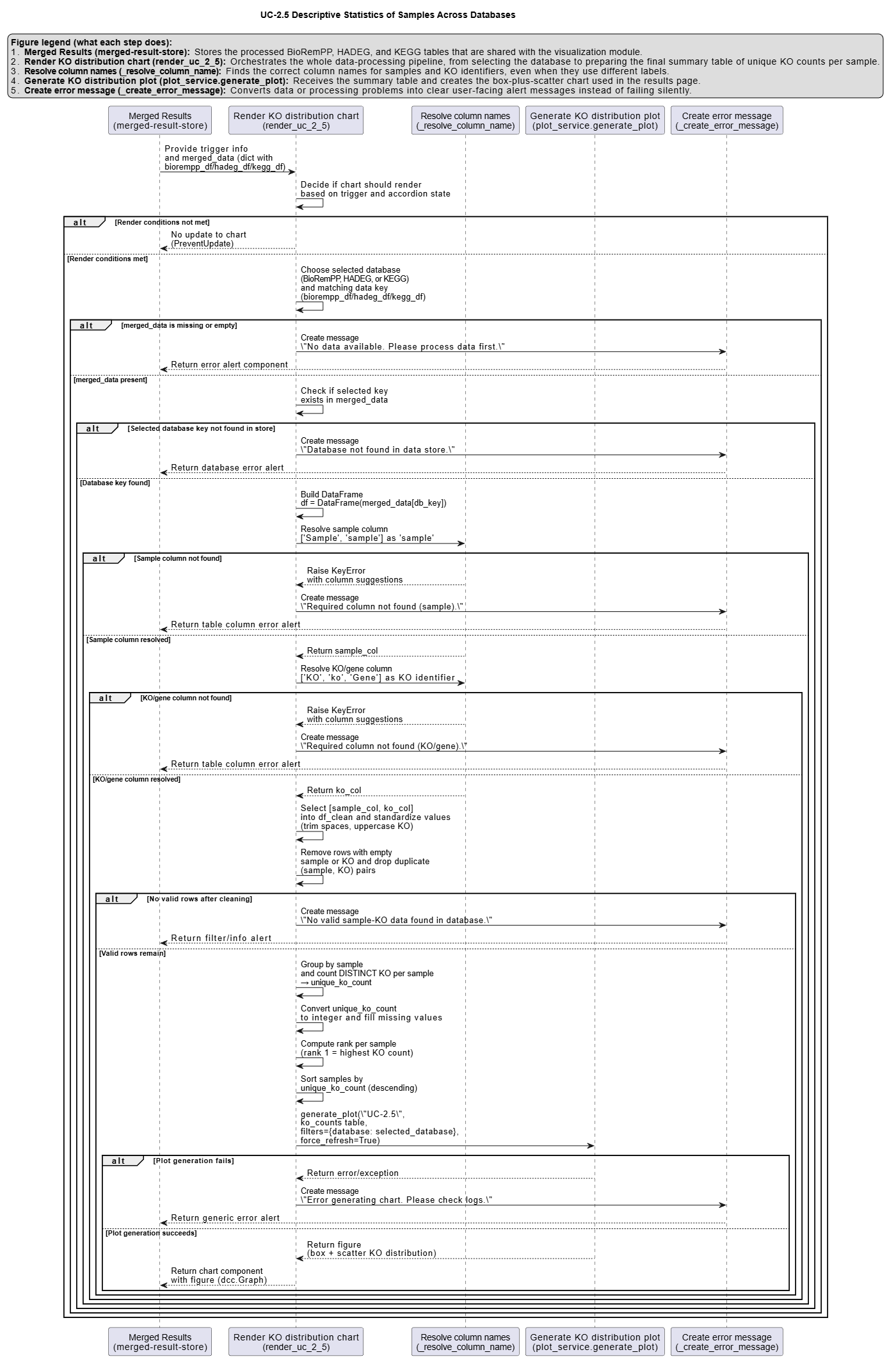
Representative Output
The image below illustrates a representative output generated by this use case using the example dataset.
Click on the image to enlarge and explore details.
Interpretation and Key Messages
- Comparing Distributions Across Databases By toggling between BioRemPP, HADEG, and KEGG, users can compare how KO annotation counts are distributed:
- A higher median in one database may suggest broader average annotation coverage per sample in that source.
-
A wider IQR or longer whiskers could indicate more variability in KO annotation counts among samples for that database.
-
Identifying Database-Specific Outliers Samples that appear as outliers (points far above or below the box) in one database but not in others may reflect a specific focus of that annotation source, warranting closer examination of which KO categories drive the difference.
-
Assessing Annotation Scope and Focus Databases with narrow, tightly clustered distributions (short boxes and whiskers) may have more uniform annotation depth or a focused scope, while broader distributions may correspond to more heterogeneous annotation coverage. Comparing spread and central tendency across databases can provide insights into differences in curation strategy and scope.
Reproducibility and Assumptions
-
Input Format
The analysis assumes semicolon-delimited tables for each database, each containing at leastsampleand a KO identifier column (koorGene). -
KO Column Handling
The code dynamically resolves whether the KO identifiers are stored underkoorGeneand treats both as equivalent sources of KO IDs. -
Uniqueness Definition KO annotation count is defined as the count of unique KO identifiers per sample. Multiple occurrences of the same KO within a sample (e.g., via multiple genes or compounds) are counted only once.
-
Jitter and Determinism
The horizontal jitter applied to sample points is seeded to produce a stable layout for a given dataset, so the same input data yields identical visual arrangements across runs. The box plot itself is a deterministic statistical summary of theunique_ko_countdistribution.
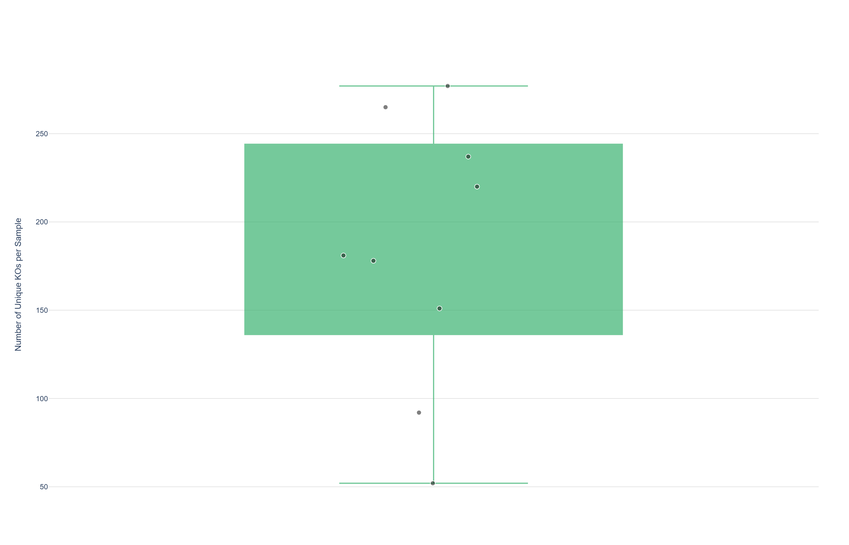
Activity diagram of the use case
Click on the image to enlarge and explore details.