UC-3.1 — Principal Component Analysis of Samples by Functional Profile
Module: 3 – System Structure: Clustering, Similarity, and Co-occurrence
Visualization type: PCA scatter plot (samples in KO-based functional space)
Primary inputs: BioRemPP results table with sample and ko columns
Primary outputs: Sample coordinates on principal components (PC1, PC2)
Scientific Question and Rationale
Question: How do the samples cluster or separate based on their overall KO annotation profiles, and which samples are the most similar or distinct in their KO annotation patterns?
This use case applies Principal Component Analysis (PCA) to visualize high-dimensional annotation relationships among biological samples. Each sample is characterized by its KEGG Orthology (KO) annotation profile. PCA projects these high-dimensional KO annotation profiles into a two-dimensional space defined by the first two principal components, which capture the major axes of annotation variation. This can facilitate the identification of annotation-based clusters, gradients, and outliers in a compact and interpretable way.
Data and Inputs
- Primary data source:
BioRemPP_Results.xlsx or BioRemPP_Results.csv - Key columns:
sample– identifier for each biological sampleko– KEGG Orthology identifier associated with the sample- Accepted format: semicolon-delimited text table (
.txtor.csv) - Derived structure: binary presence/absence matrix with:
- rows = samples
- columns = unique KOs
- cell = 1 if the sample has the KO, 0 otherwise
Analytical Workflow
-
Data Loading
The primary results table (BioRemPP_Results.xlsx or BioRemPP_Results.csv) is loaded into memory. -
Matrix Construction
A binary presence/absence matrix is constructed where: - rows correspond to Samples,
- columns correspond to unique KOs, and
-
each cell is set to
1if the sample possesses that KO and0otherwise.
This step converts categorical functional data into a numerical matrix suitable for PCA. -
Data Scaling
The binary matrix is standardized using aStandardScaler(mean-centering and scaling to unit variance). This ensures that all KO features contribute comparably to the PCA, regardless of their overall frequency. -
PCA Computation
PCA is performed on the scaled matrix to reduce dimensionality. The first two principal components (PC1 and PC2), which explain the largest fractions of variance in the KO space, are retained for visualization. -
Rendering
The samples are plotted as a scatter plot in the PC1–PC2 plane: - each point represents a Sample, and
- its coordinates correspond to the sample's scores on PC1 (X-axis) and PC2 (Y-axis).
How to Read the Plot
-
Points (Samples)
Each point in the scatter plot represents an individual Sample. -
Axes (Principal Components)
- The X-axis corresponds to Principal Component 1 (PC1).
-
The Y-axis corresponds to Principal Component 2 (PC2).
Axis labels typically include the percentage of total variance explained by each component (e.g., "PC1 (35% variance)"). -
Proximity and Distance The distance between two points may reflect their KO annotation similarity:
- samples that lie close together may have more similar KO annotation profiles,
- samples far apart may differ more strongly in the presence/absence of KOs that load heavily on PC1 and/or PC2.
Representative Output
The image below illustrates a representative output generated by this use case using the example dataset.
Click on the image to enlarge and explore details.
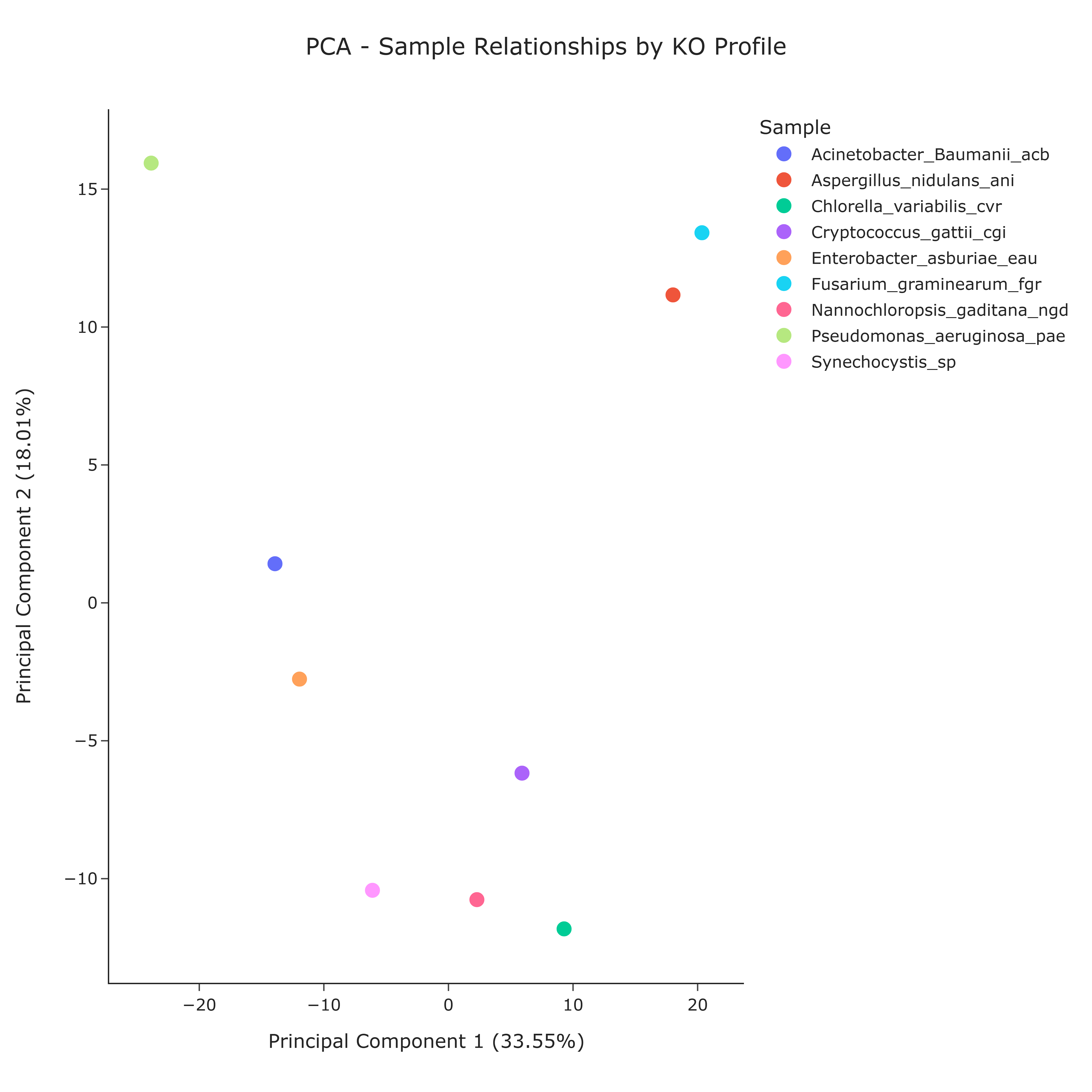
Interpretation and Key Messages
-
KO Annotation Clusters Groups of points that cluster together may indicate sets of samples with similar KO annotation profiles. These patterns could correspond to samples that share comparable KO annotation repertoires and may warrant further investigation.
-
KO Annotation Divergence and Axes of Variation Separation of samples along PC1 or PC2 may indicate the main directions of KO annotation divergence in the dataset. For example:
- separation along PC1 may suggest that the KOs with high loadings on PC1 are key discriminators between those sample groups,
-
similar reasoning applies to PC2.
-
Outliers Samples positioned far from the main clusters might be considered annotation outliers, carrying unusually distinct KO annotation profiles. These may represent samples with particularly narrow or broad annotation patterns and could warrant focused investigation.
Reproducibility and Assumptions
-
Input Format
The analysis assumes a semicolon-delimited table containing at least the columnssampleandko. -
Binary Representation
Each(sample, ko)combination is treated as a presence/absence event. Multiple occurrences of the same KO within a sample (e.g., multiple genes encoding the same KO) are collapsed into a single presence (1). -
Standardization
The PCA is performed on a standardized version of the presence/absence matrix (mean-centered and scaled to unit variance). This is a standard prerequisite for PCA when features differ in frequency or scale. -
Variance-Based Interpretation
PCA captures linear combinations of KOs that explain variance in the dataset. It does not directly model nonlinear relationships or interaction effects, which may be addressed by complementary methods in other use cases.
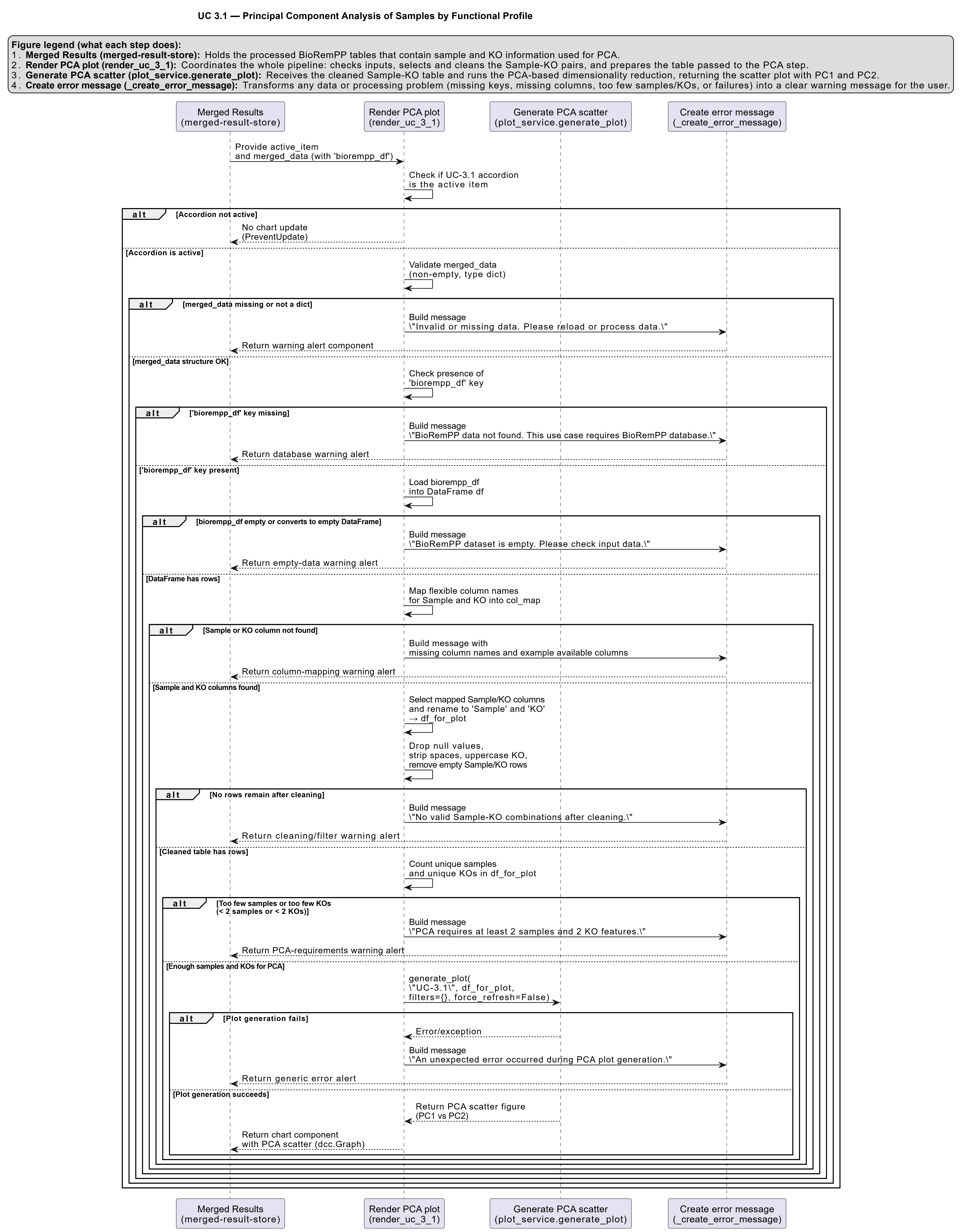
Activity diagram of the use case
Click on the image to enlarge and explore details.