UC-3.3 — Hierarchical Clustering of Samples by Functional Profile¶

Module: 3 – System Structure: Clustering, Similarity, and Co-occurrence
Visualization type: Interactive dendrogram (hierarchical clustering in KO space)
Primary inputs: BioRemPP results table with sample and ko columns
Primary outputs: Hierarchical clustering tree (linkage matrix and dendrogram) of samples based on KO profiles

Scientific Question and Rationale¶

Question: How do samples group together in a hierarchical structure based on the similarity of their KO annotation profiles, and how do different clustering algorithms and distance metrics affect these relationships?

This use case provides an interactive framework for exploring hierarchical relationships among biological samples based on their KEGG Orthology (KO) annotation profiles. By constructing a dendrogram from a KO-based presence/absence matrix, the visualization can reveal nested groupings of samples with similar KO annotation patterns. Users can dynamically change the distance metric and clustering method, making it possible to assess the robustness and sensitivity of inferred annotation-based groupings to different analytical choices.

Data and Inputs¶

• Primary data source: BioRemPP_Results.xlsx or BioRemPP_Results.csv
• Key columns:
• sample – identifier for each biological sample
• ko – KEGG Orthology identifier associated with the sample
• Accepted format: semicolon-delimited text table (.txt or .csv)
• Derived structure: binary presence/absence matrix with:
• rows = samples
• columns = unique KOs
• cell = 1 if the sample has that KO, 0 otherwise

Analytical Workflow¶

1. Data Loading
   The primary results table (BioRemPP_Results.xlsx or BioRemPP_Results.csv) is loaded into memory.

2. Matrix Construction
   A binary presence/absence matrix is constructed where:

3. rows correspond to Samples,
4. columns correspond to unique KOs, and

5. each cell is set to 1 if the sample possesses the KO and 0 otherwise.
   This matrix serves as the basis for all distance calculations.

6. Interactive Parameter Selection
   The user selects two key parameters via dropdown menus:

7. Distance Metric – the function used to quantify dissimilarity between sample profiles (e.g., jaccard, euclidean).

8. Clustering Method – the linkage algorithm used to iteratively merge clusters (e.g., average, ward).

9. Hierarchical Clustering
   Using the selected distance metric and clustering method:

10. a pairwise distance matrix between samples is computed, and

11. a linkage matrix is generated, encoding the steps by which samples and clusters are successively merged into a hierarchical tree.

12. Rendering
    The linkage matrix is rendered as an interactive dendrogram:

13. samples appear as leaves,
14. branches represent cluster merges, and
15. branch lengths reflect the chosen distance metric.

How to Read the Plot¶

• Dropdown Menus
  Use the dropdown menus to choose:
• the Distance Metric (e.g., jaccard, euclidean), and

• the Clustering Method (e.g., average, ward).
  The dendrogram updates automatically when parameters are changed.

• Leaves (Sample Labels)
  The labels at the ends of the branches (leaves) correspond to individual Samples.

• Branches and Horizontal Axis (Distance)
  The horizontal axis represents dissimilarity:

• branches that join closer to the left (with short horizontal distances) connect more similar samples or clusters,

• merges farther to the right indicate higher dissimilarity between the clusters being joined.

• Tree Topology
  The overall shape of the tree shows how samples aggregate into clusters at different levels of similarity.

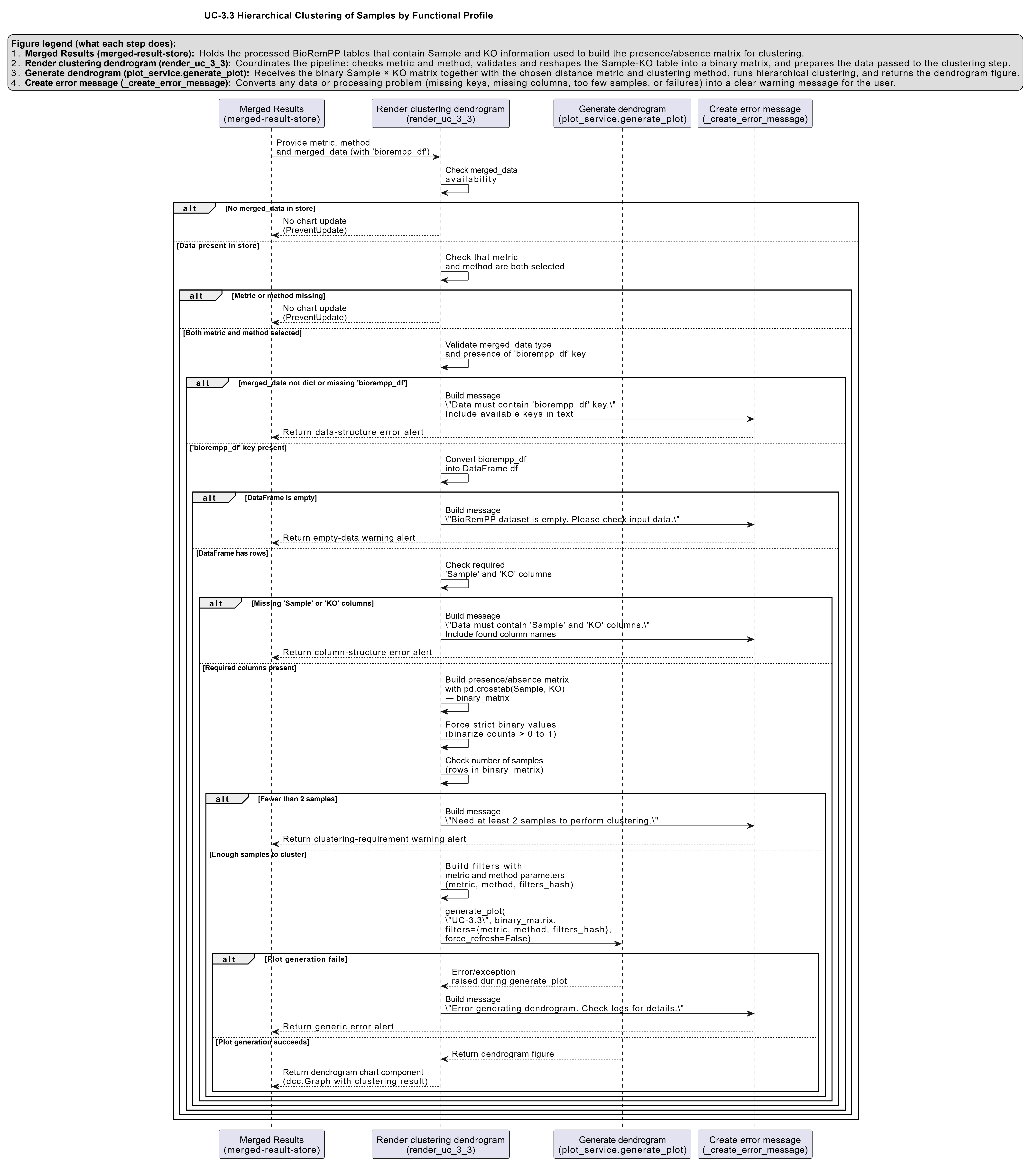
Representative Output¶

The image below illustrates a representative output generated by this use case using the example dataset.

Click on the image to enlarge and explore details.

Interpretation and Key Messages¶

• KO Annotation Clusters Groups of samples joined by short branches may form clusters with highly similar KO annotation profiles. These clusters could represent samples sharing comparable KO annotation repertoires and may be worth investigating together.

• Hierarchical Relationships The dendrogram encodes relationships at multiple scales:

• small, tight subclusters may reflect fine-grained KO annotation similarity,

• higher-level merges (farther to the right) can reveal broader divisions between major annotation-based groups.

• Robustness Across Metrics and Methods By switching distance metrics and clustering methods, users can evaluate the stability of observed clusters:

• clusters that appear consistently across different metrics/methods may correspond to more robust annotation-based groupings,

• clusters that appear only under specific parameter combinations might reflect more method-dependent structure.

• Metric Suitability
  For binary presence/absence data, metrics such as Jaccard distance are often well-suited, as they quantify dissimilarity based on shared vs. unique features. Methods like Ward's linkage require compatible metrics (e.g., Euclidean), which can influence both tree shape and interpretation.

Reproducibility and Assumptions¶

• Input Format
  The analysis assumes a semicolon-delimited table containing at least the columns sample and ko.

• Binary Representation
  Each (sample, ko) combination is reduced to a presence/absence signal. Multiple occurrences of the same KO within a sample are treated as a single presence.

• Parameter Dependence
  The dendrogram's topology is highly dependent on the choice of distance metric and clustering method:

• some combinations are mathematically incompatible (e.g., ward linkage requires a Euclidean-like metric),

• users should ensure that selected combinations are appropriate for the data type.

• Interpretation Scope The dendrogram reflects similarity in KO annotation profiles, not expression levels, gene copy numbers, or kinetic properties. These additional dimensions would require experimental validation and complementary analyses.

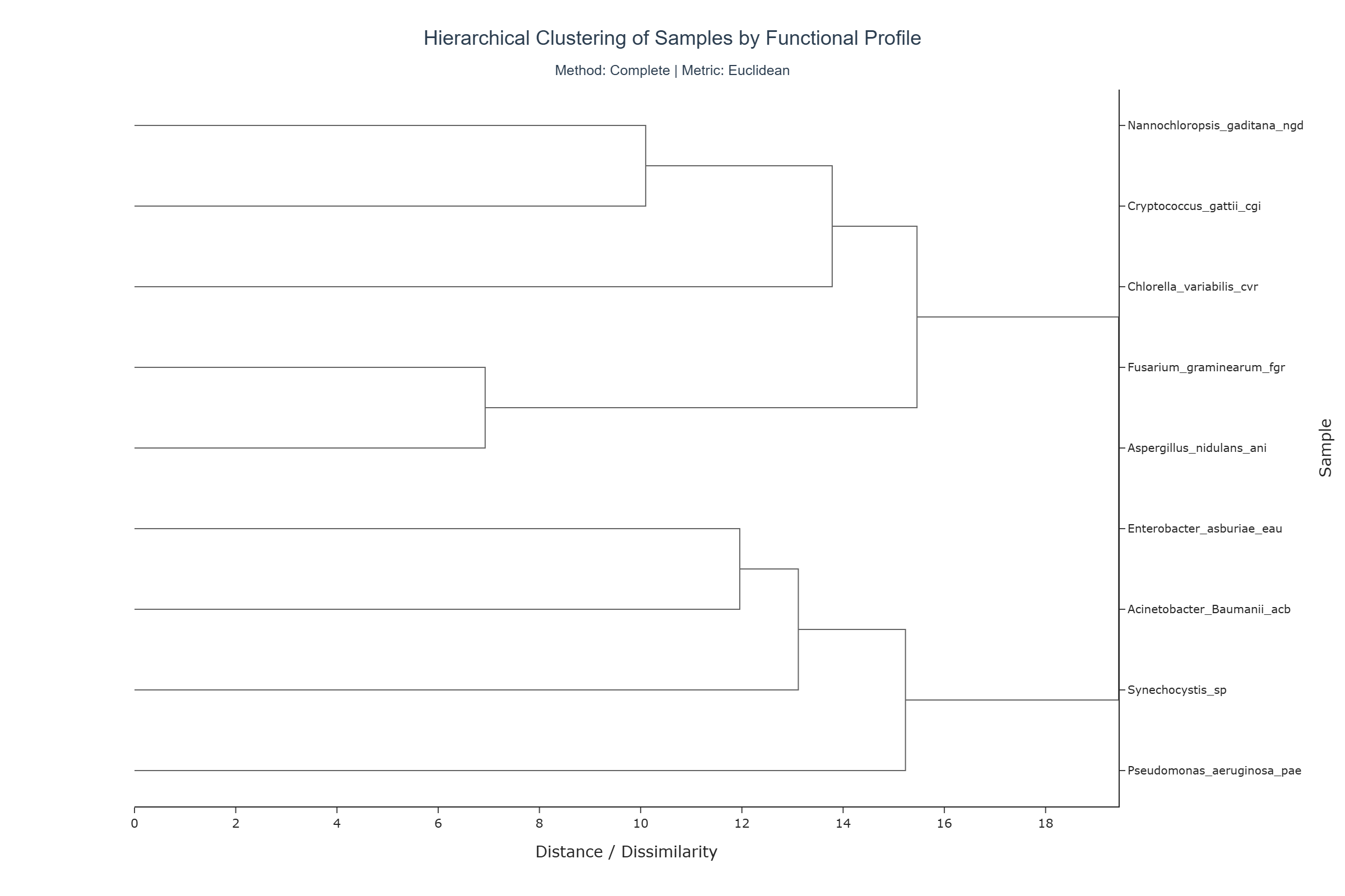
Activity diagram of the use case¶

Click on the image to enlarge and explore details.