UC-3.7 — Compound Co-occurrence Across Samples¶

Module: 3 – System Structure: Clustering, Similarity, and Co-occurrence
Visualization type: Compound × compound correlogram (co-occurrence heatmap)
Primary inputs: BioRemPP results table with sample and compoundname columns
Primary outputs: Pairwise co-occurrence (similarity) matrix of compounds across samples

Scientific Question and Rationale¶

Question: Which chemical compounds tend to co-occur in the same sample annotations, and what might this pattern suggest about shared annotation contexts, co-contamination scenarios, or chemical similarity?

This use case investigates compound co-annotation patterns across all biological samples. By examining how often pairs of compounds appear together within the same sample, the analysis constructs a compound-by-compound correlogram that maps compound co-occurrence patterns in the annotation data. These patterns may suggest shared annotation contexts or chemical groupings, though experimental validation is needed to confirm any mechanistic or environmental linkage.

Data and Inputs¶

Primary data source: BioRemPP_Results.xlsx or BioRemPP_Results.csv
Key columns:
sample – identifier for each biological sample
compoundname – name (or identifier) of the chemical compound associated with the sample
Accepted format: semicolon-delimited text table (.txt or .csv)
Derived structure: binary presence/absence matrix with:
rows = samples
columns = unique compound names
cell = 1 if the compound is associated with that sample, 0 otherwise

Analytical Workflow¶

Data Loading
The primary results table (BioRemPP_Results.xlsx or BioRemPP_Results.csv) is loaded into memory.
Matrix Construction
A binary presence/absence matrix is constructed where:
rows correspond to Samples,
columns correspond to unique compound names, and
each cell is 1 if the compound is associated with that sample and 0 otherwise.
Correlation Calculation
A compound-by-compound similarity matrix is computed by correlating the presence/absence vectors for each pair of compounds (columns). Typically:
the Pearson correlation coefficient is calculated between each pair of compound columns,
the resulting value quantifies the tendency of two compounds to be present (or absent) together across the set of samples.
Rendering
The resulting compound-by-compound correlation matrix is rendered as a heatmap (correlogram):
both axes list the same set of compounds,
cell colors encode correlation values, and
a color bar indicates the numerical range of correlation coefficients.

How to Read the Plot¶

X-axis and Y-axis (Compounds)
Both axes represent the unique Compound Names found in the dataset. The cell at row i, column j shows the co-occurrence relationship between Compound i and Compound j.
Cell Color
The color of each cell encodes the correlation coefficient between the presence/absence profiles of the two compounds across samples:
warm colors (e.g., reds) indicate high positive correlation (frequent co-occurrence),
neutral colors indicate weak or no association,
cool colors (e.g., blues) indicate negative correlation, if present.
Color Scale
A diverging color scale is typically used:
warm colors highlight strong co-occurrence,
cool colors highlight anti-correlation or mutual exclusion.
The main diagonal is always at the maximum value, since each compound is perfectly correlated with itself.

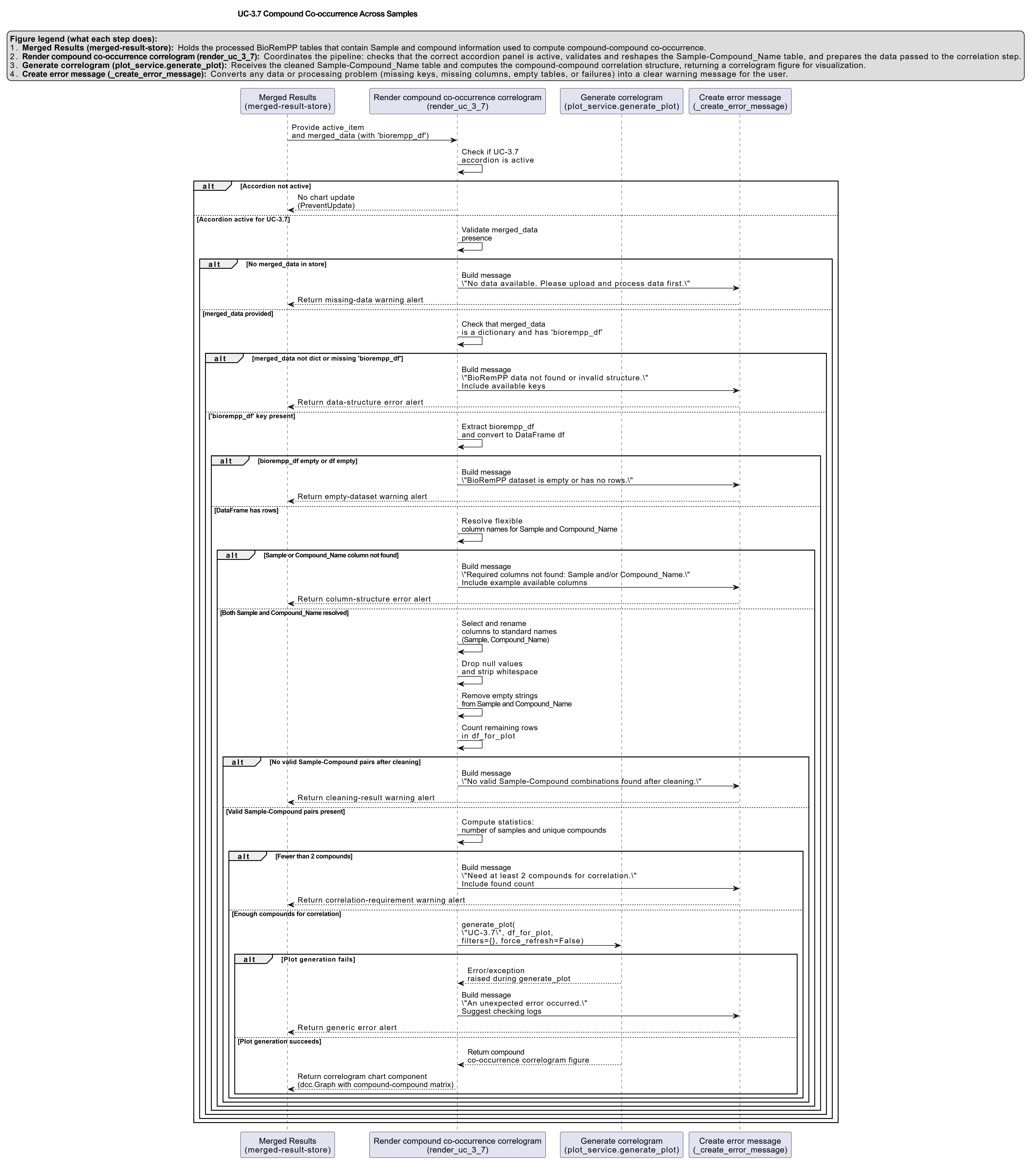
Representative Output¶

The image below illustrates a representative output generated by this use case using the example dataset.

Click on the image to enlarge and explore details.

Interpretation and Key Messages¶

Compound Co-occurrence Clusters Brightly colored blocks off the main diagonal may identify clusters of compounds that frequently co-occur across samples. These patterns could reflect:
Shared annotation context: compounds annotated together in the database (e.g., within the same pathway entries).
Co-contamination patterns: pollutants commonly co-annotated across environmental samples.
Chemical structural similarity: structurally related compounds that share annotation patterns in BioRemPP.
Distinct Compound Groups The large-scale structure of the heatmap can reveal distinct compound groupings within the annotation data:
separate warm-colored regions may correspond to different compound subsets or chemical classes,
boundaries between regions may indicate compound sets that are rarely co-annotated together.
Hypothesis Generation Co-occurrence patterns can generate hypotheses about:
pathway connectivity (which compounds may share annotation in the same metabolic routes),
compound sets that may benefit from joint investigation or monitoring. All hypotheses require experimental validation.

Reproducibility and Assumptions¶

Input Format
The analysis assumes a semicolon-delimited table containing at least the columns sample and compoundname.
Binary Representation
Co-occurrence is computed from binary presence/absence vectors. Multiple occurrences of the same compound within a single sample are treated as a single presence (1).
Similarity Metric
Associations between compounds are quantified using the Pearson correlation coefficient applied to binary vectors, capturing linear co-variation of presence/absence patterns. While widely used, other measures of association (e.g., Jaccard similarity) may be explored in complementary analyses.
Interpretation Scope The correlogram captures co-occurrence patterns in the annotation data, not causality. Compounds that co-occur frequently in annotations are candidates for shared annotation contexts, co-contamination scenarios, or chemical similarity, but additional biochemical or environmental evidence is needed to confirm any mechanistic relationships.

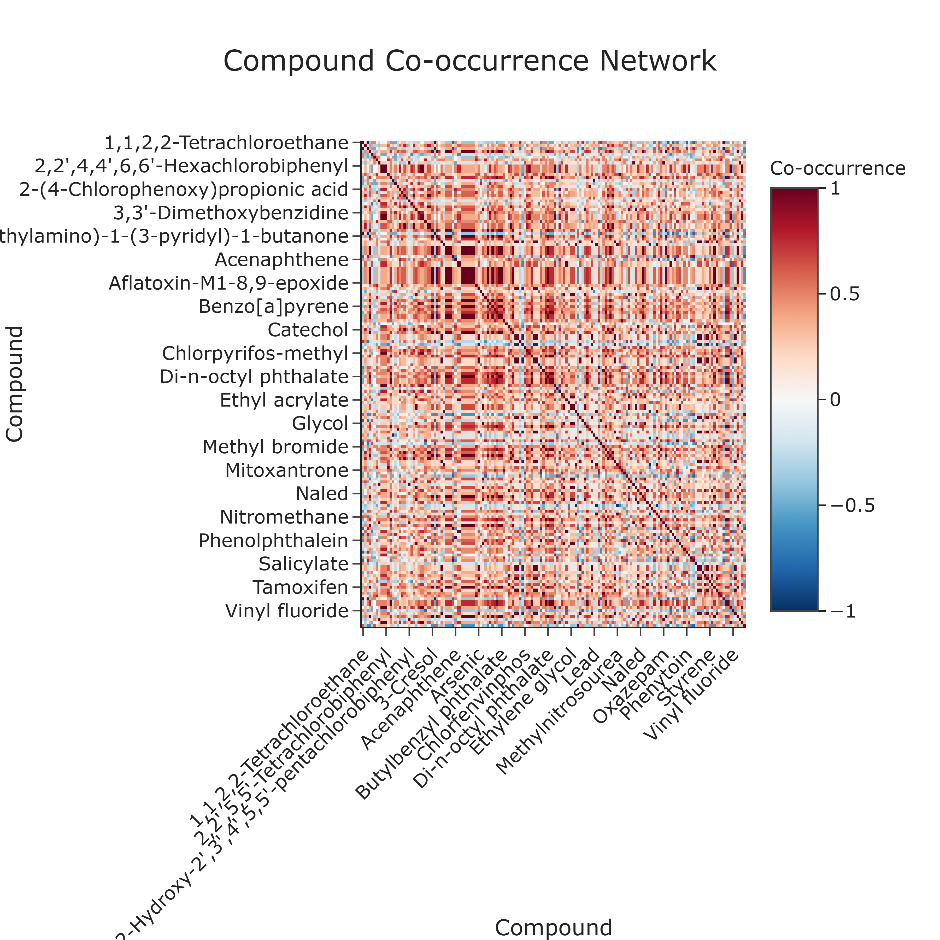
Activity diagram of the use case¶

Click on the image to enlarge and explore details.