UC-5.4 — Gene–Compound Interaction Network¶

Module: 5 – Modeling Interactions of Samples, Genes, and Compounds
Visualization type: Bipartite network graph (genes ↔ compounds)
Primary inputs: BioRemPP results table with genesymbol and compoundname columns
Primary outputs: Gene–compound interaction network (nodes, edges, node degree/centrality)

Scientific Question and Rationale¶

Question: What is the overall structure of the interaction network between genes and chemical compounds, and which entities may act as central "hubs" connecting disparate functions?

This use case builds a bipartite co-annotation network linking all detected genes to the chemical compounds with which they are co-annotated across the biological samples. By examining the topology of this network, the analysis may identify highly connected hubs and densely connected modules, which could reveal broadly co-annotated genes and widely co-annotated chemical targets. This network-level view complements sample- and pathway-level analyses by potentially exposing how gene–compound co-annotations are distributed across the dataset.

Data and Inputs¶

Primary data source: BioRemPP_Results.xlsx or BioRemPP_Results.csv
Key columns:
genesymbol – gene symbol or identifier
compoundname – name (or identifier) of the associated chemical compound
Accepted format: semicolon-delimited text table (.txt or .csv)
Derived structures:
node set of genes
node set of compounds
edge list of observed gene–compound interactions

Analytical Workflow¶

Data Loading
The primary results table (BioRemPP_Results.xlsx or BioRemPP_Results.csv) is loaded from its semicolon-delimited format.
Graph Construction (Bipartite Network)
A bipartite graph is built using a network library (e.g., networkx):
each unique genesymbol is added as a gene node (type = "gene"),
each unique compoundname is added as a compound node (type = "compound"),
for every row in the table, an undirected edge is added between the corresponding gene and compound, representing an observed interaction.
Layout Calculation
A force-directed layout algorithm (e.g., spring_layout) is applied to compute 2D coordinates for each node:
highly connected nodes tend to be placed toward the center,
sparsely connected nodes tend to be pushed toward the periphery,
clusters of nodes naturally emerge from the optimization of edge lengths and repulsive forces.
Computation of Node Properties
For each node, the degree (number of incident edges) is calculated:
this serves as a simple hubness metric,
it is later displayed as part of the hover information.
Rendering
The network is rendered using an interactive plotting library (e.g., plotly):
nodes are plotted at their layout coordinates,
edges are drawn as straight segments between node positions,
genes and compounds receive distinct, solid colors and uniform node sizes,
hover tooltips expose node identity and degree (e.g., "Gene: gstA" — Interactions: 15).

How to Read the Plot¶

Nodes
Each point in the graph is a node representing:
a Gene (e.g., shown in one color), or
a Compound (shown in a contrasting color).
Edges
Each line (edge) between a gene and a compound represents an observed interaction:
at least one row in the results table links that gene to that compound in some sample.
Hover Information
Hovering over a node reveals:
its type and name (e.g., "Gene: gstA", "Compound: benzene"),
its number of connections (degree), reflecting how many interaction partners it has.
Spatial Structure
The spatial layout is informative but not literal:
nodes closer to the center or to each other may be more highly or densely connected,
clusters of nodes may indicate sub-networks of genes and compounds with many shared interactions.

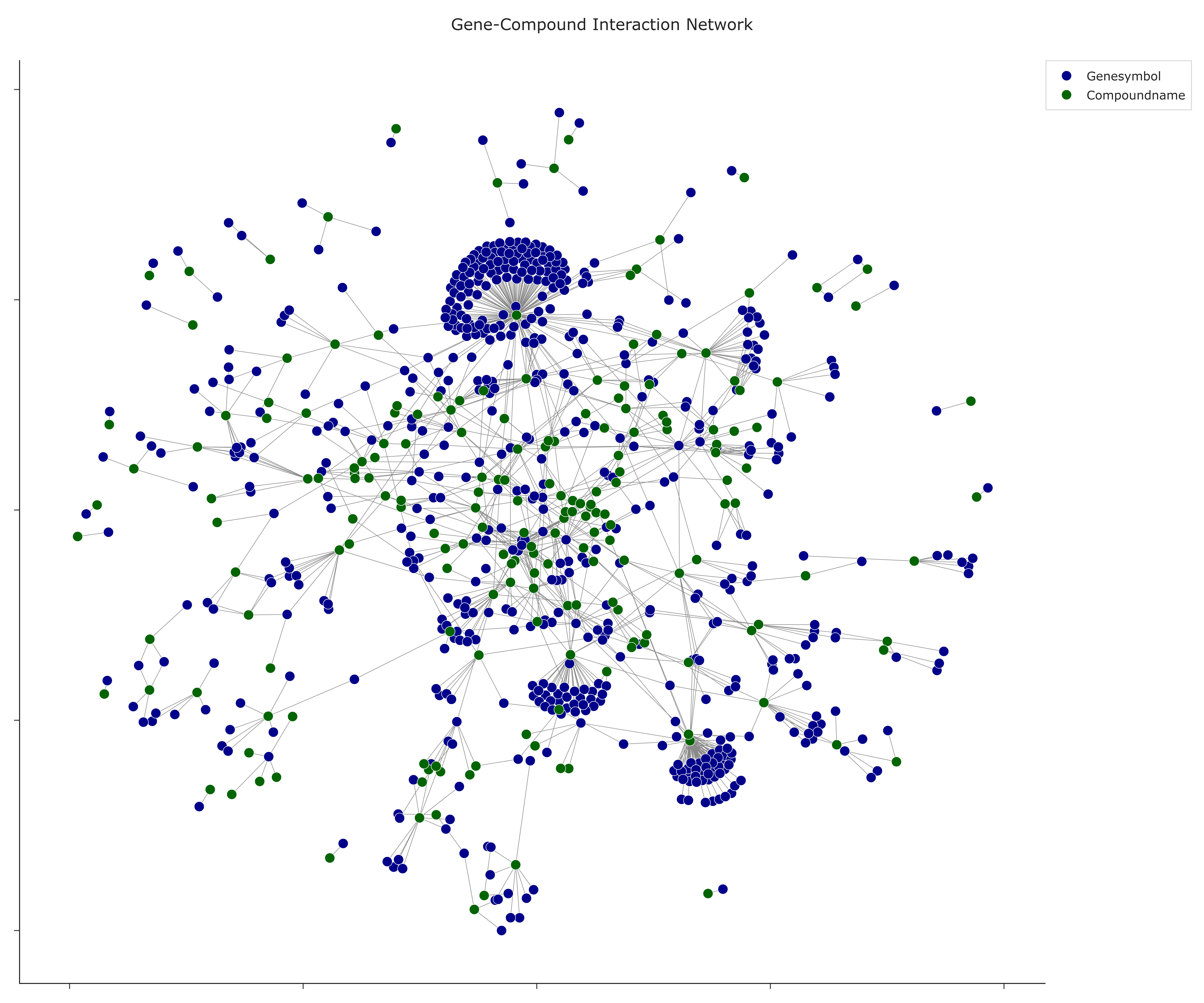
Representative Output¶

The image below illustrates a representative output generated by this use case using the example dataset.

Click on the image to enlarge and explore details.

Interpretation and Key Messages¶

Hub Nodes Nodes with high degree and central positions may be co-annotation hubs:
a gene hub is a gene co-annotated with many different compounds, which may suggest broad co-annotation coverage or annotation centrality,
a compound hub is a chemical co-annotated with many different genes, which may point to a widely annotated compound in the database.
Co-annotation Clusters Tightly packed clusters of genes and compounds may represent co-annotation groups:
sets of genes frequently co-annotated with a family of structurally related compounds,
candidate annotation patterns that could be further validated via pathway mapping or experimental data.
Peripheral Nodes Nodes located on the outer regions of the layout with few connections could be:
genes with narrow co-annotation coverage, or
compounds with limited representation in the annotation data. These elements may be relevant for niche or focused investigation scenarios.
Bridging Elements Nodes that connect otherwise separate clusters may act as annotation bridges:
a gene bridging two compound clusters could link annotation groups across chemical families,
a compound bridging gene clusters could represent a broadly co-annotated intermediate in the database.

Reproducibility and Assumptions¶

Input Format
The analysis assumes a semicolon-delimited table containing at least the columns genesymbol and compoundname.
Network Definition
The network is undirected and unweighted in this representation: an edge indicates that a gene–compound interaction exists, but does not encode interaction frequency or strength.
Node degree reflects the number of distinct partners, not the number of occurrences in the raw table.
Layout and Visual Bias
The force-directed layout (spring_layout) is stochastic but reproducible when a random seed is fixed.
Visual centrality in the plot is correlated with connectivity but is not a formal centrality metric—additional measures (e.g., betweenness, eigenvector centrality) can be computed if needed.
Interpretation Scope
The graph reveals topological patterns of interaction, not mechanistic or kinetic details:
co-connectivity may suggest potential functional relationships but does not itself establish biochemical mechanisms,
further validation using pathway databases, structural information, or experimental data is required to confirm mechanistic roles.

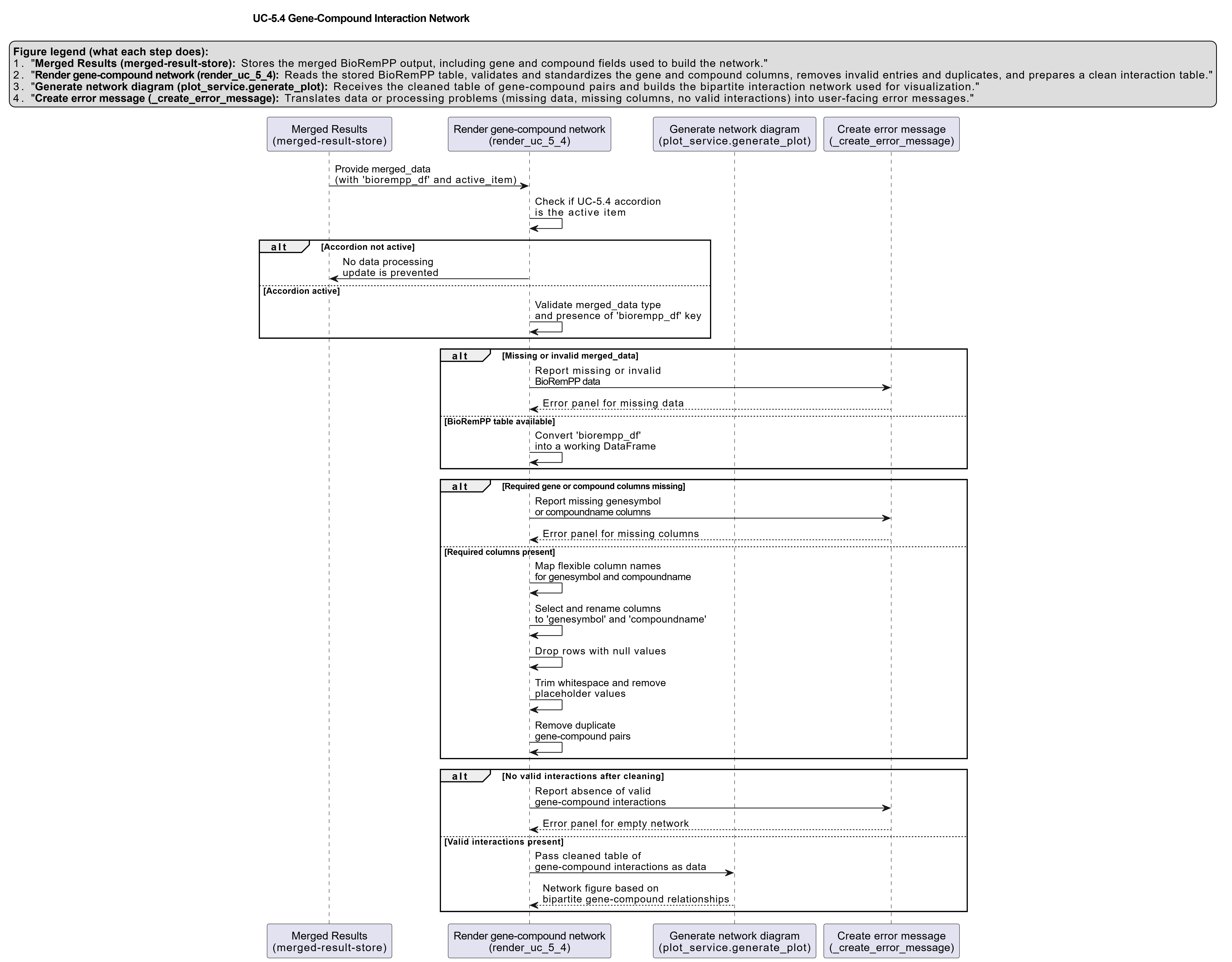
Activity diagram of the use case¶

Click on the image to enlarge and explore details.