UC-5.5 — Gene–Gene Interaction Network (Based on Shared Compounds)
Module: 5 – Modeling Interactions of Samples, Genes, and Compounds
Visualization type: Weighted gene–gene network (shared-compound edges, force-directed layout)
Primary inputs: BioRemPP results table with genesymbol and compoundname columns
Primary outputs: Gene–gene interaction network weighted by number of shared compounds; node-level connectivity (degree)
Scientific Question and Rationale
Question: Which genes share the most compound co-annotations across samples, and what co-annotation structure do these gene–gene relationships form?
This use case examines gene–gene co-annotation overlap by identifying which genes are co-annotated with overlapping sets of chemical compounds across all biological samples. Genes that share many compound co-annotations could warrant investigation as potential functional partners, though experimental validation is required. By constructing a gene–gene network where edges represent shared compound co-annotations and edge weights encode the number of these shared annotations, the analysis may highlight co-annotation clusters, highly connected hub genes, and potential bridge genes that connect distinct annotation subsets.
Data and Inputs
- Primary data source:
BioRemPP_Results.xlsx or BioRemPP_Results.csv - Key columns:
genesymbol– gene symbol or identifiercompoundname– name (or identifier) of the chemical compound associated with that gene in at least one sample- Accepted format: semicolon-delimited text table (
.txtor.csv) - Derived structures:
- mapping of each gene to its set of unique compounds,
- weighted gene–gene edge list based on the count of shared compounds.
Analytical Workflow
-
Data Loading
The primary results table (BioRemPP_Results.xlsx or BioRemPP_Results.csv) is loaded from its semicolon-delimited format. -
Gene-to-Compound Mapping
For each uniquegenesymbol, a compound set is constructed: - all unique
compoundnameentries associated with that gene are collected into a set, -
this set represents the compound co-annotation profile of that gene.
-
Graph Construction (Gene–Gene Network)
A network graph is built where: - each unique gene is added as a node,
-
all unique pairs of genes are evaluated; for each pair:
- the intersection of their compound sets is computed,
- if the intersection is non-empty, an edge is added between the two genes,
- the edge weight is set to the number of shared unique compounds.
-
Layout and Styling
A force-directed layout is used to compute node positions: - genes with many strong connections tend to be drawn closer to one another, forming clusters,
- sparsely connected genes are placed closer to the periphery.
Node attributes are then computed: - degree (number of connected gene neighbors) is calculated for each node,
-
this degree is mapped to node color to highlight highly connected genes.
-
Rendering
The network is rendered as an interactive plot: - nodes represent individual genes,
- edges represent gene–gene links based on shared compounds,
- edge thickness is proportional to edge weight (number of shared compounds),
- node color is proportional to degree (number of gene neighbors), with a color bar indicating the scale.
How to Read the Plot
- Nodes (Genes)
Each point in the graph is a Gene Symbol: - the position is determined by the force-directed layout,
-
the color of a node encodes its degree (how many other genes it is connected to).
-
Edges (Gene–Gene Links) Each line between two nodes represents a shared compound co-annotation link:
- two genes share at least one common compound co-annotation,
-
the thickness of the edge is proportional to the number of shared compound co-annotations (edge weight).
-
Color Scale for Nodes
A color bar indicates the range of node degrees: - nodes with brighter/warmer colors correspond to high-degree genes (hubs),
-
nodes with cooler or darker colors correspond to lower-degree genes.
-
Overall Structure
The spatial arrangement may reflect the network's modular organization: - dense clusters could indicate groups of genes with many shared compound partners,
- sparsely connected or isolated nodes might indicate more specialized or infrequent relationships.
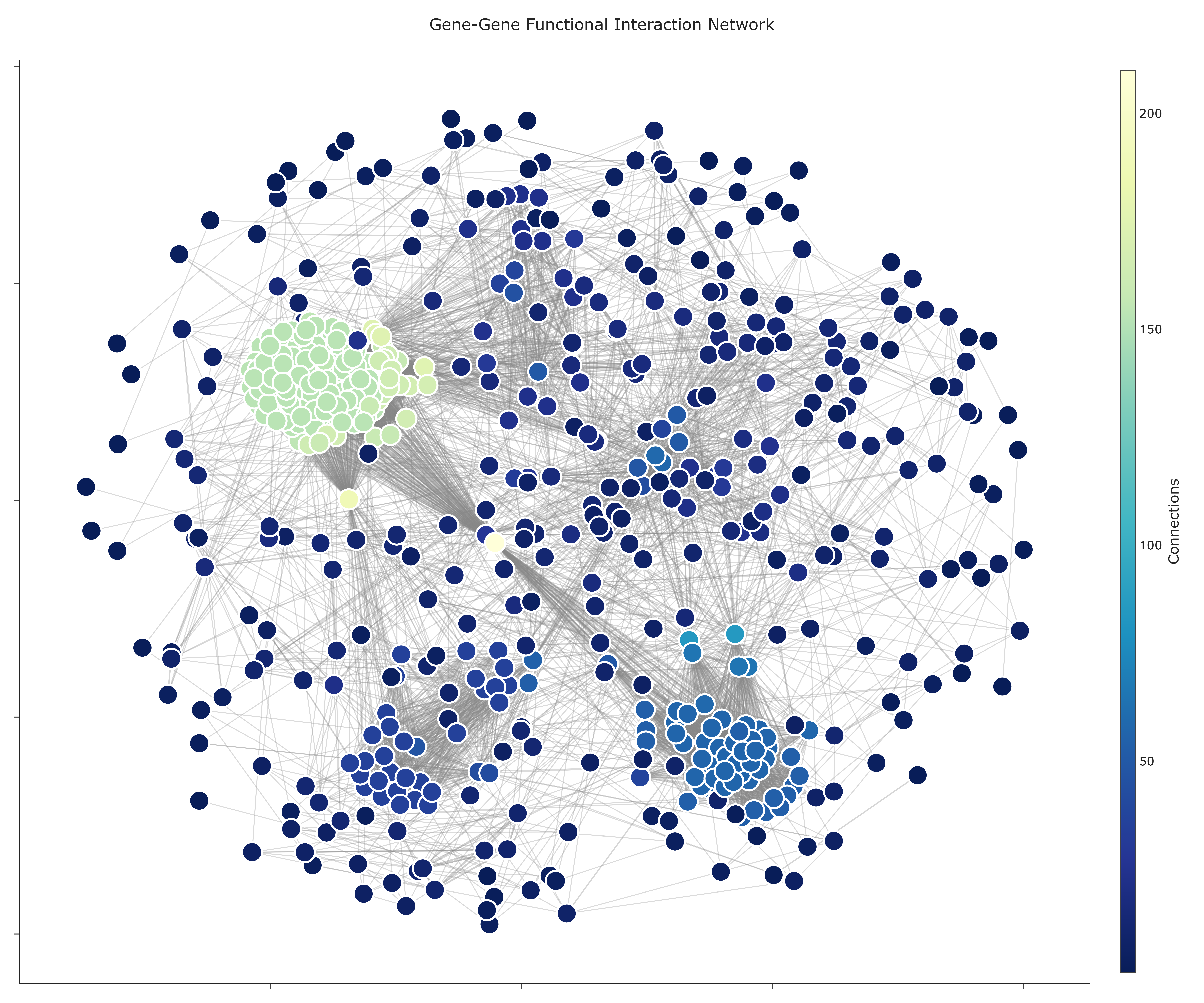
Representative Output
The image below illustrates a representative output generated by this use case using the example dataset.
Click on the image to enlarge and explore details.
Interpretation and Key Messages
- Co-annotation Clusters Dense clusters of interconnected nodes may represent gene co-annotation groups:
- genes in the same cluster tend to share many compound co-annotations,
-
they are candidates for belonging to related annotation contexts, though pathway membership requires experimental validation.
-
Hub Genes Brightly colored, centrally located nodes with many edges may be broadly co-annotated hub genes:
- they share compound co-annotations with many other genes,
-
they could represent genes with broad annotation coverage across many compounds in the database.
-
Bridge Genes Genes that connect otherwise distinct clusters may act as annotation bridges:
- they could link different annotation groups or chemical families,
-
they represent genes whose co-annotation patterns span multiple compound subsets.
-
Peripheral Genes Nodes on the network's periphery with few connections may represent narrowly co-annotated genes:
- they could be relevant for rare or niche compound co-annotations,
- they may still be important in targeted investigation scenarios even if not highly connected.
Reproducibility and Assumptions
-
Input Format
The analysis assumes a semicolon-delimited table containing at least the columnsgenesymbolandcompoundname. -
Link Definition
- A link between two genes is defined by the presence of at least one shared compound co-annotation in their annotation sets.
- Edge weight is the number of shared unique compound co-annotations.
-
Node color reflects gene–gene connectivity (degree), not the total number of gene–compound co-annotations.
-
Network Properties
- The network is typically treated as undirected and weighted: directionality is not inferred, but the strength of association is encoded in edge weights.
-
The layout is based on a force-directed algorithm that can be made reproducible by fixing a random seed.
-
Interpretation Scope
- The network captures association patterns inferred from shared compound targets; it does not directly encode regulatory direction, reaction stoichiometry, or kinetic parameters.
- Co-connectivity should be interpreted as hypothesis-generating evidence for functional relationships that require additional biochemical, genomic, or regulatory validation.
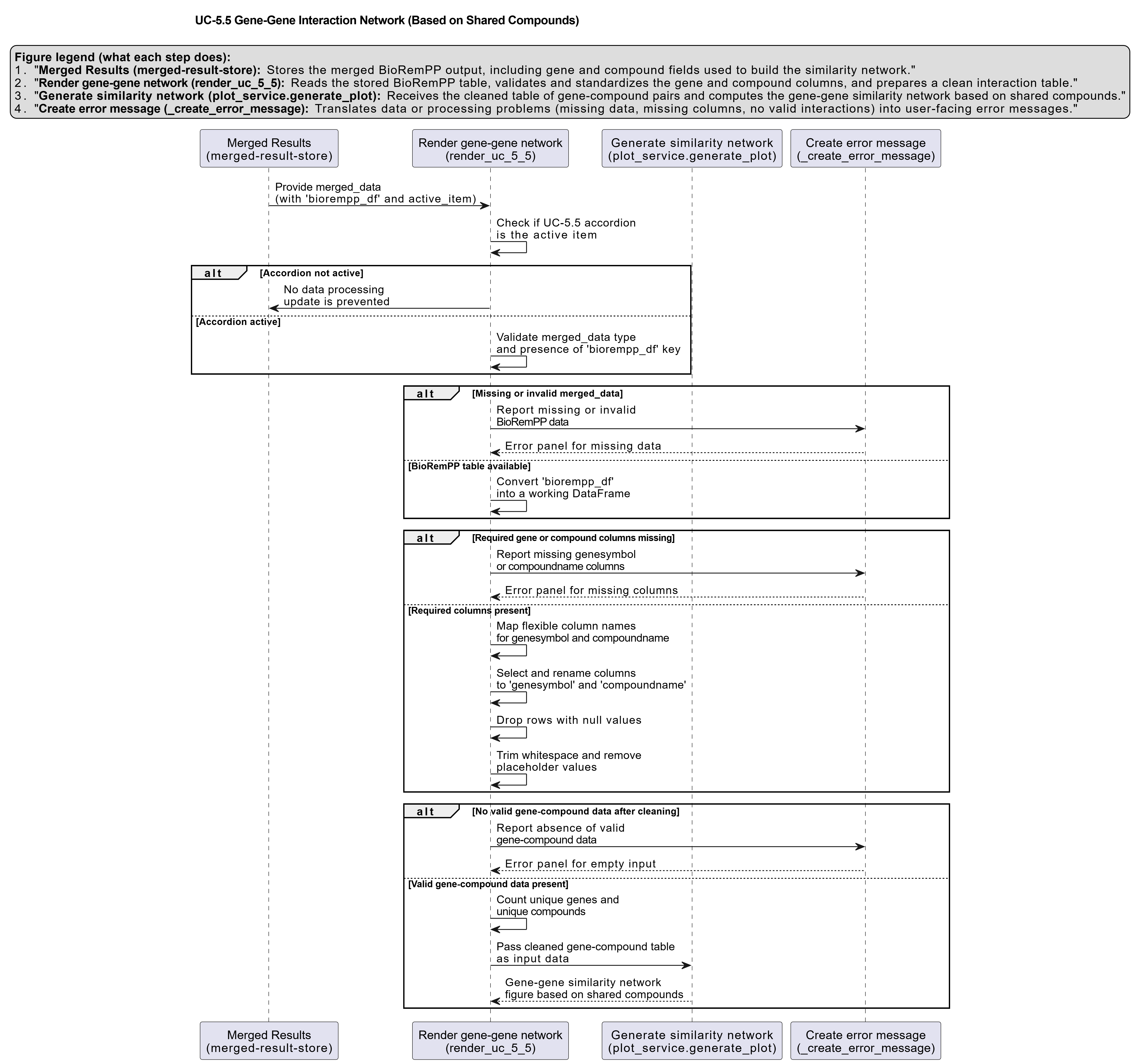
Activity diagram of the use case
Click on the image to enlarge and explore details.